01
Newton’s second law
ODE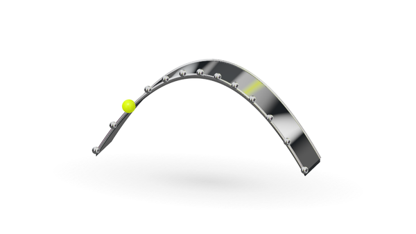
Force sets the acceleration.

A few rules. Endless forms.
TAP TO REFORMAll 39 studies
Force sets the acceleration.
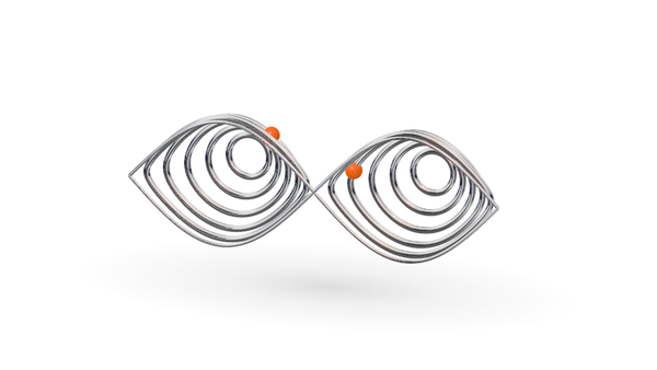
The path of stationary action.pendulum: angle vs angular speed
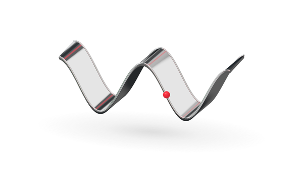
Restoring force: pure oscillation.
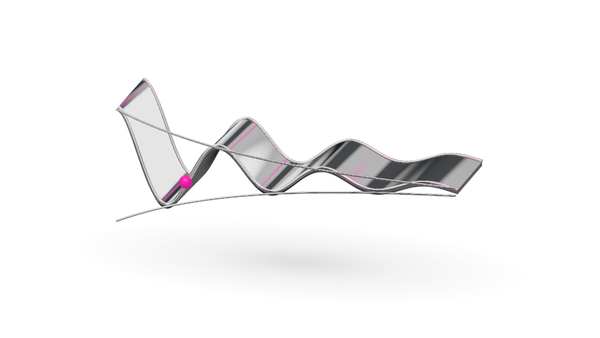
Friction drains the swing away.
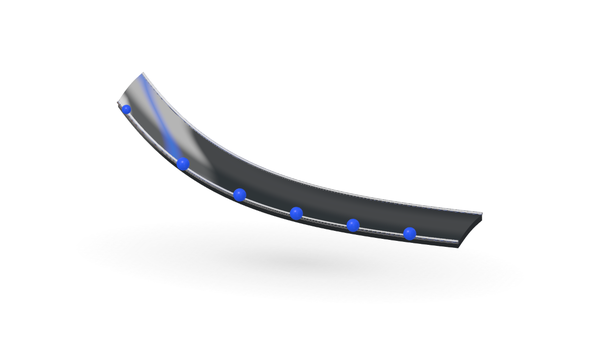
Rate of decay ∝ amount left.
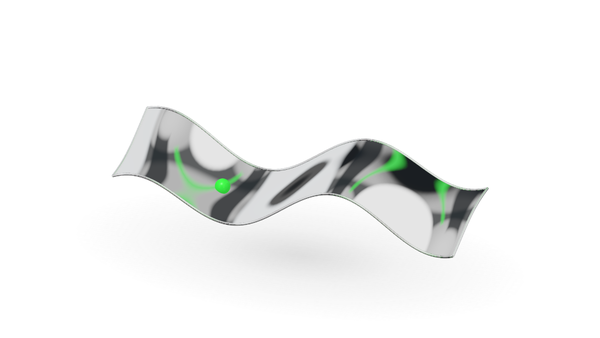
Disturbances travel at speed c.
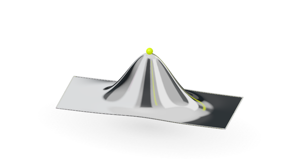
Hot spots spread and smooth out.
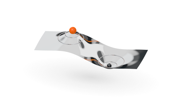
Charges set the potential.
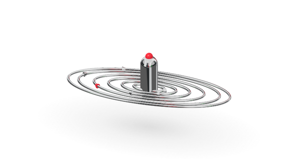
Changing B makes E circulate.
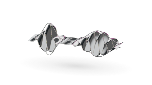
How a quantum state evolves.
Newton’s second law for a fluid.
Mass-energy curves spacetime.
The FLRW metric describes homogeneous, isotropic spatial slices. The scale factor a(t) changes their size; k = +1, 0, −1 selects positive, zero or negative spatial curvature. The chrome expansion here is a sculptural illustration, not a fitted cosmological history.
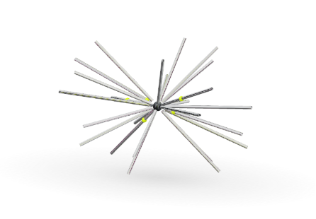
Eight ways to arrive. Or leave.
Exact exponential trajectories of three-dimensional linear systems. The spiral family has eigenvalues α ± iω and β; the signs of α and β select attraction or repulsion in the plane and along the axis. These eight examples cover the supplied hyperbolic families, not every possible equilibrium. Display axes are scaled for the sculpture.
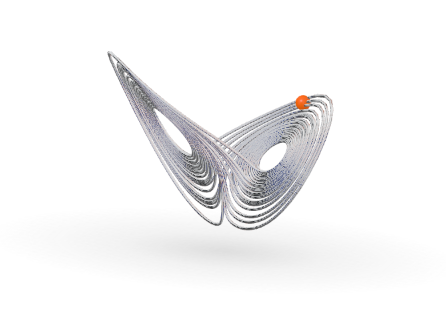
A familiar shape. An unfamiliar return.
A finite numerical trajectory of the Lorenz equations with σ = 10, ρ = 28 and β = 8/3. Fourth-order Runge–Kutta integration uses a step of 0.005 after discarding the initial transient. The bead follows the same sampled trajectory; its finite exhibition cycle restarts. Display axes are scaled independently.
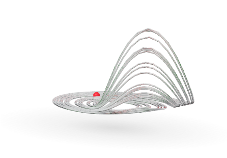
Round. Round. Suddenly elsewhere.
Rössler's system with a = b = 0.2 and c = 5.7. A fourth-order Runge–Kutta trajectory, step 0.018, follows a discarded transient. The bead loops over the finite sampled record. Axes are scaled independently to reveal the lifted fold.
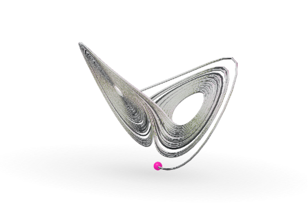
Almost the same is not the same.
Two Lorenz solutions start at (1, 1, 1) and (1.000001, 1, 1), with identical parameters and integration steps. Chrome and dark paths show the complete finite records; the tether joins equal simulation times. The 42-second cycle restarts from the two initial conditions. Numerical divergence illustrates sensitivity, not a quantitative Lyapunov-exponent measurement.
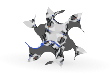
Every opening leads somewhere.
The zero level of a trigonometric nodal approximation to the gyroid. One periodic cell is shown; its mean curvature is close to, but not identically, zero. The fluorescent edge follows the same level set.
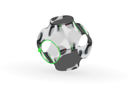
Rooms without walls.
A nodal approximation to Schwarz’s primitive minimal surface, clipped to one periodic cell. The displayed cosine level set preserves the connected passages; it is not an exact zero-mean-curvature surface.
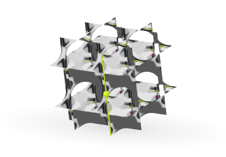
A different kind of diamond.
A trigonometric nodal approximation to the Schwarz diamond surface. Its two labyrinths have tetrahedral connectivity. The rendered zero set approximates the minimal surface; the cubic crop is a viewing boundary.
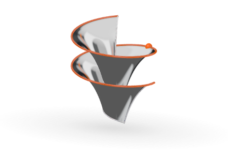
A trumpet that took a wrong turn.
Dini’s parametric surface has constant Gaussian curvature K = −1/(a² + b²). A finite regular patch is shown, ending before v = π/2, where this parametrization becomes singular. The coloured rim follows the outer parameter curve.
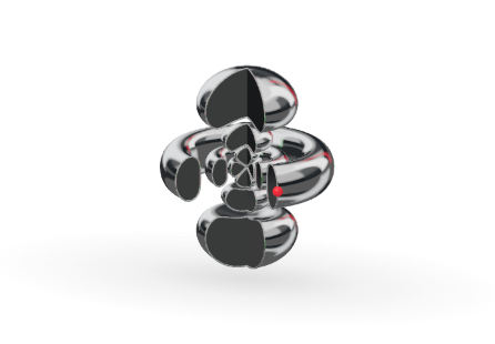
A silence between each shell.
A constant-amplitude surface of the n = 5, ℓ = 2, m = 0 hydrogen state. The cutaway exposes three radial bands. R₅₂ ∝ ρ² exp(−ρ/2)(ρ² − 14ρ + 42), with ρ = 2r/(5a₀); its radial nodes are ρ = 7 ± √7. The light traces the section; it is not an electron.
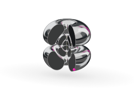
The same atom. Another opening.
A cutaway level set of |R₅₂Y₂¹|. The angular magnitude is proportional to |sin θ cos θ|; the complex phase winds once around the axis. Both radial nodes are preserved. This is the complex m = 1 state, rather than a real d-orbital combination. The surface is a selected amplitude level, not a hard atomic boundary.
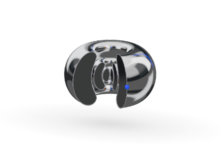
Three rings. Nothing to hold.
A cutaway level set of |R₅₂Y₂²|, with angular magnitude proportional to sin² θ and complex phase exp(2iφ). The shared 5d radial function supplies two spherical nodes. All three studies use the same radial scale and amplitude threshold after normalising each angular factor to its peak. Chrome expresses the surface; it does not encode probability colour.
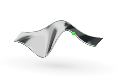
One touch changes the shape.
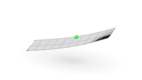
The two edges show ψ₀(q) = exp(−q²/2) and qψ₀(q). The connecting sheet makes the operator's action visible; its depth is a comparison coordinate. Amplitudes use separate display scales. This is multiplication of a wavefunction, not a simulation of a position measurement.
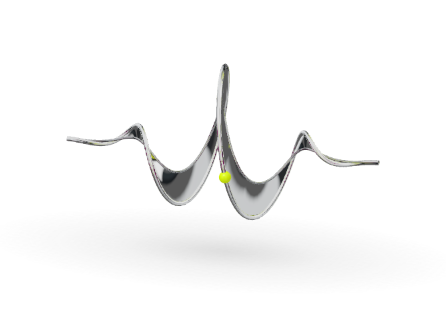
A twist hidden in the slope.
For ψ(q) = exp(−q²/2 + ikq), with k = 3.2 and ℏ = 1, p̂ψ = (k + iq)ψ exactly. Height and depth carry the real and imaginary components. The ribbon joins ψ and p̂ψ/k at separate display scales; the light reads the curve rather than tracking a particle.
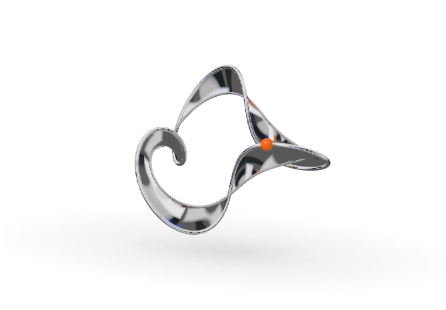
A whole number of turns.
The ring state ψ(φ) = exp(3iφ) satisfies L̂zψ = 3ℏψ. Its complex amplitude becomes the minor radius and height of a toroidal ribbon, with its two edges in the ratio 1:3. The phase returns after one full turn. Density on the physical ring is uniform; the sculptural folds represent phase.
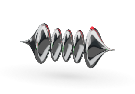
Everything moves. The shape stays.
The n = 4 harmonic-oscillator state, ψ₄ ∝ H₄(q)exp(−q²/2), has four nodes and energy E₄ = 9ℏω/2. Revolving |ψ₄| creates this amplitude envelope. Its density stays fixed while its common phase evolves as exp(−iE₄t/ℏ). The revolving light indicates phase, not electron motion.
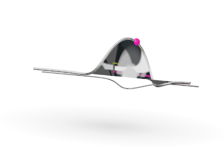
A wave that keeps its word.
An exact coherent state of H = (p² + q²)/2 in oscillator units. Its centre is q₀ = 1.3 cos τ and momentum p₀ = −1.3 sin τ; ψ ∝ exp[−(q−q₀)²/2 + ip₀(q−q₀/2) − iτ/2]. The fan shows complex amplitude. The fine lower curve shows |ψ|². Display time is τ = 0.85 + 0.36t.
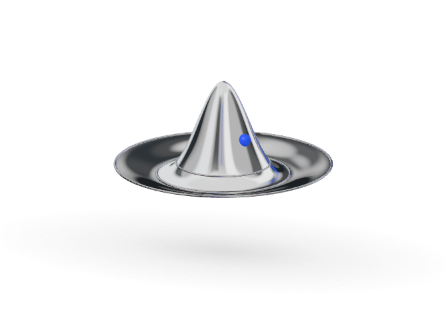
Curvature leaves a crown.
For the two-dimensional Gaussian ψ = exp(−r²/2) and ℏ = m = 1, T̂ψ = (1 − r²/2)exp(−r²/2). The silver sheet plots that signed amplitude, including its zero at r = √2. It is an operator acting on a state, not a local kinetic-energy density; negative amplitude does not imply negative kinetic energy.
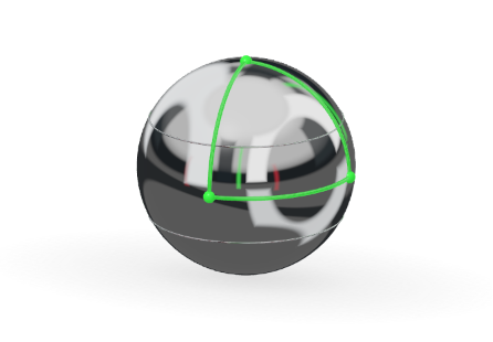
Three right angles. One triangle.
The three edges are quarter great circles on a sphere, enclosing one octant: their angles sum to 270°. The excess over 180° equals area divided by radius squared. This two-dimensional model illustrates positive spatial curvature, not a picture of the entire universe.
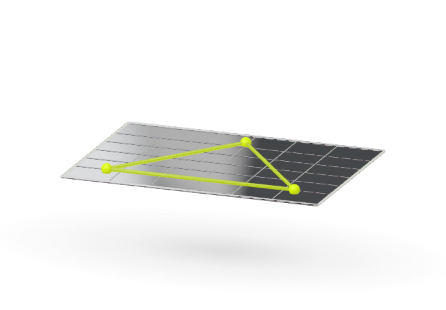
A familiar kind of straight.
A planar triangle with straight geodesic edges. Its interior angles sum to 180°. The plane is a local two-dimensional analogue of the flat spatial slices in an FLRW cosmology; flatness alone does not determine global topology.
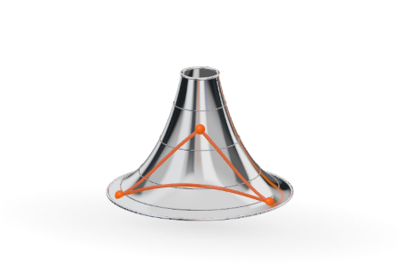
Less than a half-turn.
A finite patch of a pseudosphere, with constant Gaussian curvature K = −1/a². The highlighted edges are hyperbolic geodesics, mapped from circles orthogonal to the upper-half-plane boundary. Their angles total less than 180°. This is a local model, not a complete embedding of hyperbolic space.
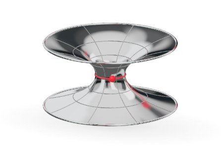
Two sides of a possibility.
A catenoid embedding of the equatorial, constant-time slice of the Ellis/Morris–Thorne model, with shape function b(r) = b₀²/r and zero redshift function. This hypothetical traversable solution requires exotic stress-energy; the surface is a spatial diagram, not a tunnel observed in nature.
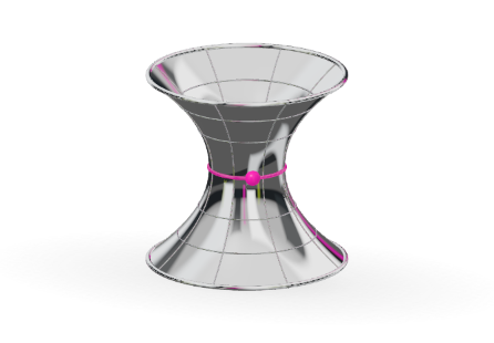
A bridge with no crossing.
The time-symmetric spatial slice of the maximally extended Schwarzschild solution, with rₛ = 2GM/c². The two Flamm paraboloids meet at the horizon. This hypothetical bridge is nontraversable: the embedding does not provide a path for a traveller between the exterior regions.
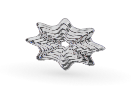
Together, without being identical.
A Fourier-contour sculpture inspired by the supplied symmetry/coherence quartet. Repeated integer modes produce rotational symmetry; mixed coprime modes disturb it. Coherence here means one connected composition versus nine separate forms, not a measured optical or quantum coherence field. The folded depth is a sculptural mapping of the contours.
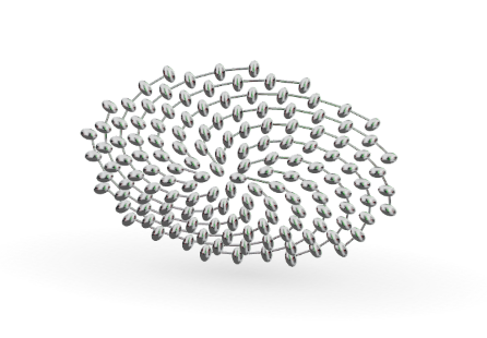
One turn. A hundred and forty-four possibilities.
Vogel-style golden-angle placement, θₙ = nπ(3 − √5), with a half-index radial offset to avoid crowding the centre. The plane is domed and scaled for display. Fine rails connect seeds thirteen indices apart, revealing one family of parastichies. The bead steps through insertion order; this is a geometric packing model, not a biological growth simulation.
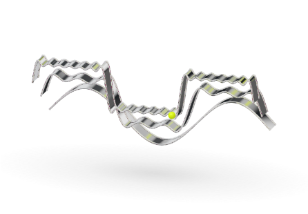
One voice. Three voices. Seven.
Successive partial sums of the odd-harmonic Fourier series, with amplitudes proportional to 1/(2k + 1). All three use the same travelling phase. Their heights and depths are separated for comparison. The overshoot near each emerging discontinuity is the Gibbs phenomenon; these are finite smooth sums, not exact square waves.
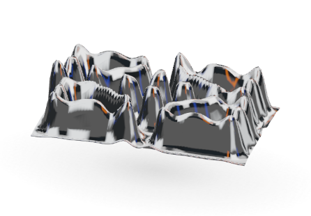
A pattern with no pattern-maker.
A live two-species Gray–Scott simulation on a 68 × 68 periodic grid. Du = 0.16, Dv = 0.08, F = 0.035 and k = 0.062; forward Euler with unit grid spacing and unit time steps follows a 1,800-step seed evolution. Height maps the second concentration. Numerical concentrations are bounded to [0, 1]; the metal is a visual encoding, not a simulated material.
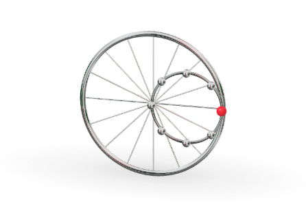
Circles, conspiring to make a straight line.
The Tusi couple is the 2:1 hypocycloid: a point on the rolling inner circle moves along a diameter. The visible inner circle constructs the accented bead's path. The remaining beads are rotated copies with angular frequencies in the ratio 1:2:3:4:5:6:7:8 and staggered phases; they do not share one rolling wheel. Listening is optional: each turning point can become a note.